Measurement and uncertainties
1.2.1 State the fundamental units in the SI system.
Many different types of measurements are made in physics. In order to provide a clear and concise set of data, a specific system of units is used across all sciences. This system is called the International System of Units (SI from the French "Système International d'unités").
The SI system is composed of seven fundamental units:
| Quantity | Unit name | Unit symbol |
| mass | kilogram | kg |
| time | second | s |
| length | meter | m |
| temperature | kelvin | K |
| Electric current | ampere | A |
| Amount of substance | mole | mol |
| Luminous intensity | candela | cd |
Note that the last unit, candela, is not used in the IB diploma program.
1.2.2 Distinguish between fundamental and derived units and give examples of derived units.
In order to express certain quantities we combine the SI base units to form new ones. For example, if we wanted to express a quantity of speed which is distance/time we write m/s (or, more correctly m s-1). For some quantities, we combine the same unit twice or more, for example, to measure area which is length x width we write m2.
Certain combinations or SI units can be rather long and hard to read, for this reason, some of these combinations have been given a new unit and symbol in order to simplify the reading of data.
For example: power, which is the rate of using energy, is written as kg m2 s-3. This combination is used so often that a new unit has been derived from it called the watt (symbol: W).
Below is a table containing some of the SI derived units you will often encounter:
| SI derived unit | Symbol | SI base unit | Alternative unit |
| newton | N | kg m s-2 | - |
| joule | J | kg m2 s-2 | N m |
| hertz | Hz | s-1 | - |
| watt | W | kg m2 s-3 | J s-1 |
| volt | V | kg m2 s-3 A-1 | W A-1 |
| ohm | Ω | kg m2 s-3 A-2 | V A-1 |
| pascal | Pa | kg m-1 s-2 | N m-2 |
1.2.3 Convert between different units of quantities.
Often, we need to convert between different units. For example, if we were trying to calculate the cost of heating a litre of water we would need to convert between joules (J) and kilowatt hours (kW h), as the energy required to heat water is given in joules and the cost of the electricity used to heat the water is a certain price per kW h.
If we look at table 1.2.2, we can see that one watt is equal to a joule per second. This makes it easy to convert from joules to watt hours: there are 60 second in a minutes and 60 minutes in an hour, therefor, 1 W h = 60 x 60 J, and one kW h = 1 W h / 1000 (the k in kW h being a prefix standing for kilo which is 1000).
1.2.4 State units in the accepted SI format.
There are several ways to write most derived units. For example: meters per second can be written as m/s or m s-1. It is important to note that only the latter, m s-1, is accepted as a valid format. Therefor, you should always write meters per second (speed) as m s-1 and meters per second per second (acceleration) as m s-2. Note that this applies to all units, not just the two stated above.
1.2.5 State values in scientific notation and in multiples of units with appropriate prefixes.
When expressing large or small quantities we often use prefixes in front of the unit. For example, instead of writing 10000 V we write 10 kV, where k stands for kilo, which is 1000. We do the same for small quantities such as 1 mV which is equal to 0,001 V, m standing for milli meaning one thousandth (1/1000).
When expressing the units in words rather than symbols we say 10 kilowatts and 1 milliwatt.
A table of prefixes is given on page 2 of the physics data booklet.
1.2.6 Describe and give examples of random and systematic errors.
Random errors
A random error, is an error which affects a reading at random.
Sources of random errors include:
- The observer being less than perfect
- The readability of the equipment
- External effects on the observed item
Systematic errors
A systematic error, is an error which occurs at each reading.
Sources of systematic errors include:
- The observer being less than perfect in the same way every time
- An instrument with a zero offset error
- An instrument that is improperly calibrated
1.2.7 Distinguish between precision and accuracy.
Precision
A measurement is said to be accurate if it has little systematic errors.
Accuracy
A measurement is said to be precise if it has little random errors.
A measurement can be of great precision but be inaccurate (for example, if the instrument used had a zero offset error).
1.2.8 Explain how the effects of random errors may be reduced.
The effect of random errors on a set of data can be reduced by repeating readings. On the other hand, because systematic errors occur at each reading, repeating readings does not reduce their affect on the data.
1.2.9 Calculate quantities and results of calculations to the appropriate number of significant figures.
The number of significant figures in a result should mirror the precision of the input data. That is to say, when dividing and multiplying, the number of significant figures must not exceed that of the least precise value.
Example:
Find the speed of a car that travels 11.21 meters in 1.23 seconds.
11.21 x 1.13 = 13.7883
The answer contains 6 significant figures. However, since the value for time (1.23 s) is only 3 s.f. we write the answer as 13.7 m s-1.
The number of significant figures in any answer should reflect the number of significant figures in the given data.
1.2.10 State uncertainties as absolute, fractional and percentage uncertainties.
Absolute uncertainties
When marking the absolute uncertainty in a piece of data, we simply add ± 1 of the smallest significant figure.
Example:
13.21 m ± 0.01
0.002 g ± 0.001
1.2 s ± 0.1
12 V ± 1
Fractional uncertainties
To calculate the fractional uncertainty of a piece of data we simply divide the uncertainty by the value of the data.
Example:
1.2 s ± 0.1
Fractional uncertainty:
0.1 / 1.2 = 0.0625
Percentage uncertainties
To calculate the percentage uncertainty of a piece of data we simply multiply the fractional uncertainty by 100.
Example:
1.2 s ± 0.1
Percentage uncertainty:
0.1 / 1.2 x 100 = 6.25 %
1.2.11 Determine the uncertainties in results.
Simply displaying the uncertainty in data is not enough, we need to include it in any calculations we do with the data.
Addition and subtraction
When performing additions and subtractions we simply need to add together the absolute uncertainties.
Example:
Add the values 1.2 ± 0.1, 12.01 ± 0.01, 7.21 ± 0.01
1.2 + 12.01 + 7.21 = 20.42
0.1 + 0.01 + 0.01 = 0.12
20.42 ± 0.12
Multiplication, division and powers
When performing multiplications and divisions, or, dealing with powers, we simply add together the percentage uncertainties.
Example:
Multiply the values 1.2 ± 0.1, 12.01 ± 0.01
1.2 x 12.01 = 14
0.1 / 1.2 x 100 = 8.33 %
0.01 / 12.01 X 100 = 0.083%
8.33 + 0.083 = 8.413 %
14 ± 8.413 %
Other functions
For other functions, such as trigonometric ones, we calculate the mean, highest and lowest value to determine the uncertainty range. To do this, we calculate a result using the given values as normal, with added error margin and subtracted error margin. We then check the difference between the best value and the ones with added and subtracted error margin and use the largest difference as the error margin in the result.
Example:
Calculate the area of a field if it's length is 12 ± 1 m and width is 7 ± 0.2 m.
Best value for area:
12 x 7 = 84 m2
Highest value for area:
13 x 7.2 = 93.6 m2
Lowest value for area:
11 x 6.8 = 74.8 m2
If we round the values we get an area of:
84 ± 10 m2
1.2.12 Identify uncertainties as error bars in graphs.
When representing data as a graph, we represent uncertainty in the data points by adding error bars. We can see the uncertainty range by checking the length of the error bars in each direction. Error bars can be seen in figure 1.2.1 below:
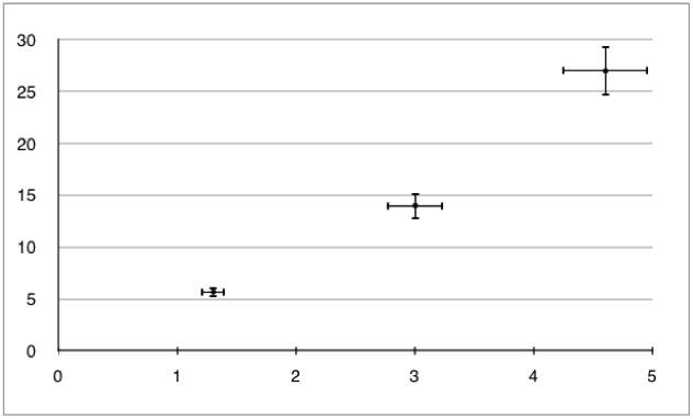
Figure 1.2.1 - A graph with error bars
1.2.13 State random uncertainty as an uncertainty range (±) and represent it graphically as an "error bar".
In IB physics, error bars only need to be used when the uncertainty in one or both of the plotted quantities are significant. Error bars are not required for trigonometric and logarithmic functions.
To add error bars to a point on a graph, we simply take the uncertainty range (expressed as "± value" in the data) and draw lines of a corresponding size above and below or on each side of the point depending on the axis the value corresponds to.
Example:
Plot the following data onto a graph taking into account the uncertainty.
| Time ± 0.2 s | Distance ± 2 m |
| 3.4 | 13 |
| 5.1 | 36 |
| 7 | 64 |
Table 1.2.1 - Distance vs Time data
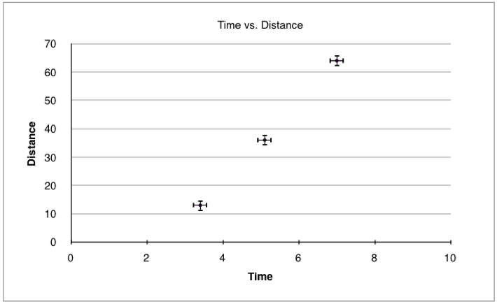
Figure 1.2.2 - Distance vs. time graph with error bars
In practice, plotting each point with its specific error bars can be time consuming as we would need to calculate the uncertainty range for each point. Therefor, we often skip certain points and only add error bars to specific ones. We can use the list of rules below to save time:
- Add error bars only to the first and last points
- Only add error bars to the point with the worst uncertainty
- Add error bars to all points but use the uncertainty of the worst point
- Only add error bars to the axis with the worst uncertainty
1.2.14 Determine the uncertainties in the gradient and intercepts of a straight- line graph.
Gradient
To calculate the uncertainty in the gradient, we simply add error bars to the first and last point, and then draw a straight line passing through the lowest error bar of the one points and the highest in the other and vice versa. This gives two lines, one with the steepest possible gradient and one with the shallowest, we then calculate the gradient of each line and compare it to the best value. This is demonstrated in figure 1.2.3 below:
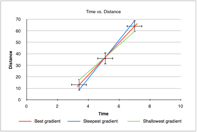
Figure 1.2.3 - Gradient uncertainty in a graph
Intercept
To calculate the uncertainty in the intercept, we do the same thing as when calculating the uncertainty in gradient. This time however, we check the lowest, highest and best value for the intercept. This is demonstrated in figure 1.2.4 below:
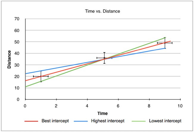
Figure 1.2.4 - Intercept uncertainty in a graph
Note that in the two figures above the error bars have been exaggerated to improve readability.